マテリアルズ・インフォマティクスにおけるデータ分析

本記事の概要

　この記事では、マテリアルズ・インフォマティクスに限った話ではないが、機械学習を行う前のデータ分析について紹介していく。
グラフは発表などでも使えるように綺麗に作成している（論文でも使える？）ので、参考までにどうぞ。
目次：

データ分析の重要性

　最近は機械学習のライブラリが発展しているため、すぐに機械学習にデータをかけて予測することができる。しかし、機械学習にかける前にデータ分析をすることで良い高い予測精度への改善ができたり、新しい相関関係などを見つけることができる。今回はそのデータ分析の実装方法をテンプレート的に紹介する。今回は、回帰予測を行うことを前提にデータ分析を行っている

データの準備

　ここで扱うデータは前記事と同じくLi-O系の化合物に関する生成エネルギーに関するものである。データ分析を行うために、事前に以下を実行しておく。以下のコードは、ライブラリのインポート、データの読み込みである。

# データ加工・処理・分析ライブラリ
import pandas as pd
import numpy as np

# 可視化ライブラリ
import matplotlib.pyplot as plt
import seaborn as sns
%matplotlib inline

#Li-O系の化合物データに関する記述子、目的変数が入っているファイル名
filename='./Li_O_atom2vec_ave_var_with_form_ene_per_atom.csv'
df = pd.read_csv(filename,index_col=0)
df.head()

目的変数に対する分析

今回は、目的変数に関して4つのデータ分析を行う。データが手に入ったら、まずやってみると良い（私は、大体この４つはやっている）。

ヒストグラムの作成

まずは、目的変数に対するヒストグラムから確認する。

#ここでは、ヒストグラムを描くための関数（サブルーティン）を作成している。
def make_hist(df,column_name,bins=100):
    #図を綺麗に書く設定
    plt.rcParams['font.family'] = 'Times New Roman' #Font
    plt.rcParams['xtick.direction'] = 'in' # x axis in
    plt.rcParams['ytick.direction'] = 'in' # y axis in 
    plt.rcParams['axes.linewidth'] = 1.0 # axis line width   

    fig = plt.figure(figsize=(6,4),dpi=100) #FIgure Size
    ax = fig.add_subplot(111) #Figure position
    output_fig = 'out.{}.png'.format(column_name) #Image name
    ax.hist(df[column_name],bins=bins,color='k')
    ax.yaxis.set_ticks_position('both')
    ax.xaxis.set_ticks_position('both')    
    ax.set_title('{} histogram'.format(column_name))
    ax.set_xlabel(column_name)
    ax.set_ylabel('Frequency')
    plt.savefig(output_fig)
    print('Mean :',round(df[column_name].mean(),4))
    print('Median :',round(df[column_name].median(),4))    
    print('output figure:',output_fig)
    plt.show()
    
column_name='formation_energy_per_atom'
make_hist(df,column_name)

>（出力）
Mean : -2.2949
Median : -2.3526
output figure: out.formation_energy_per_atom.png

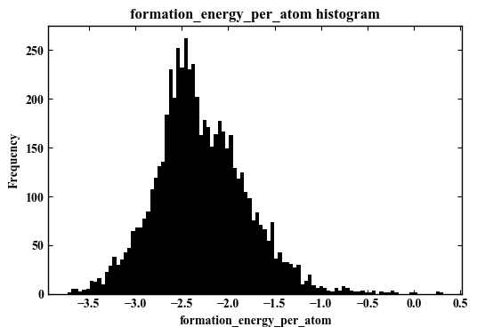
　今回の目的変数は正規分布に近い形になっていることがわかる。よって、ある程度回帰問題として解きやすいだろうと推測できる。
データが明らかに2分しているような分布だったり、偏りが非常に大きい場合はうまく回帰できない場合が多い。そのような場合は、回帰問題ではなく、分類問題に変換した方が良いかもしれない。

箱ひげ図を描く

みんながよく知っている箱ひげ図

#ここでは、箱ひげ図(Boxplot)を描くための関数（サブルーティン）を作成している。
def make_box_plot(df,column_name):
    plt.rcParams['font.family'] = 'Times New Roman'
    plt.rcParams['xtick.direction'] = 'in' # x axis in
    plt.rcParams['ytick.direction'] = 'in' # y axis in 
    plt.rcParams['axes.linewidth'] = 1.0 # axis line width       
    fig = plt.figure(figsize=(6,4))
    ax = fig.add_subplot(111)
    ax.boxplot(df[column_name])
    ax.set_title('Boxplot plot {}'.format(column_name))
    ax.set_ylabel('Count')
    ax.set_xlabel(column_name) 
    ax.yaxis.set_ticks_position('both')
    print(df[column_name].describe())

column_name='formation_energy_per_atom'
make_box_plot(df,column_name)

> （出力）
count 6033.000000
mean -2.294868
std 0.493983
min -3.732763
25% -2.610536
50% -2.352607
75% -1.989622
max 0.316142
Name: formation_energy_per_atom, dtype: float64

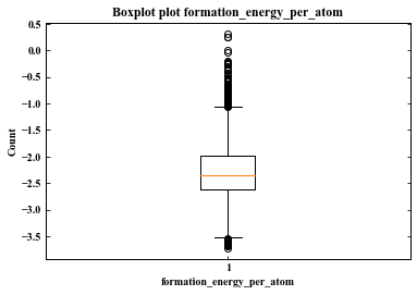
　ここでは、明らかな外れ値があるかどうかを調べている。今回は、ひどい外れ値は見当たらないと考えられる。

機器トラブルなどで桁違いに外れている値であったり、物理的におかしい値がある場合はそれらのデータを除外してから機械学習にかけた方がよいだろう。

目的変数と記述子の相関関係

目的変数と記述子の相関係数を確認する。

def feature_plot(df_corr,column_name,labelsize=18):
    plt.rcParams['font.family'] = 'Times New Roman'
    plt.rcParams['xtick.direction'] = 'in' # x axis in
    plt.rcParams['ytick.direction'] = 'in' # y axis in 
    plt.rcParams['axes.linewidth'] = 1.0 # axis line width         
    fig = plt.figure(figsize=(14,6))
    ax = fig.add_subplot(111)    
    ax.bar(df_corr.index,df_corr['formation_energy_per_atom'], color='Black', linestyle=':')
    ax.set_ylabel('Correlation coefficient between target and descriptors',fontsize=labelsize)
    ax.set_xlabel('Features',fontsize=labelsize)
    ax.yaxis.set_ticks_position('both')
    ax.set_xticklabels(df_corr.index,rotation=90,fontsize=labelsize)
    ax.set_title('Correlation between target and descriptors',fontsize=labelsize*1.2)
    plt.show()

column_name='formation_energy_per_atom'
df_corr = df.corr().iloc[:-1]
feature_plot(df_corr,column_name)

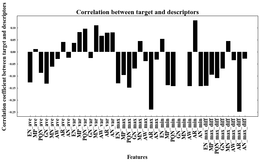
AR_max_diffが目的変数に対して、比較的大きな負の相関を持っていることがわかる。次に具体的にその相関状況を見てみる。

効きそうな記述子と目的変数の関係をさらに具体的に表示する

　全ての記述子と目的変数の散布図を作成するのは、めんどくさいし、確認するにも時間がかかる。今回は、上の分析で一番相関係数の絶対値が大きかった記述子と目的変数の関係性をみる。なお、相関係数は、一時的相関しか反映されないため、二次的相関などそのほかの相関がある可能性もあるということを頭のすみに入れておいて方が良い。

def r(x,y):
    x_ = x.mean()
    y_ = y.mean()
    return (sum((x-x_)*(y-y_)))/ (np.sqrt((np.square(x-x_).sum()*(np.square(y-y_).sum()))))
                                 
def plot(df,column1,column2,pos_x=0.9,pos_y=0.5):
    plt.rcParams['font.family'] = 'Times New Roman'
    plt.rcParams['xtick.direction'] = 'in' # x axis in
    plt.rcParams['ytick.direction'] = 'in' # y axis in 
    plt.rcParams['axes.linewidth'] = 1.0 # axis line width       
    x_max_value,y_max_value = max(df[column1]),max(df[column2])
    fig = plt.figure(figsize=(12,8),dpi=100)
    ax = fig.add_subplot(221)
    ax.scatter(df[column1],df[column2],color='k',s=5)
    ax.set_xlabel(column1)
    ax.set_ylabel(column2)
    s='r = '+str(round(r(df[column1],df[column2]),4))
    ax.text(x = x_max_value*pos_x, y = y_max_value*pos_y ,s=s)
    ax.yaxis.set_ticks_position('both')
    ax.xaxis.set_ticks_position('both')      
    ax.set_title('{} vs {}'.format(column1,column2))
    plt.show()        

column1='AR_max_diff'
column2='formation_energy_per_atom'
plot(df,column1,column2)

このグラフからは、それほど明らかな相関があるような形にはなっていないことが確認できる。　
なお、上記の関数とFor文をうまく用いれば、全ての記述子と目的変数の散布図を簡単に作成することができる。

記述子間の相関分析

記述子間の関係性も重要である。多重共線性などを確認するのにも役立つため、ぜひ確認しておいて欲しい。 記述子間の相関を全て確認するのは、非常に手間がかかりそうだが、以下のプログラムを用いることで全ての記述子間の相関をヒートマップ的に確認することができる。非常に便利なので重宝している。

plt.rcParams['font.family'] = 'Times New Roman'
plt.rcParams['xtick.direction'] = 'in' # x axis in
plt.rcParams['ytick.direction'] = 'in' # y axis in 
plt.rcParams['axes.linewidth'] = 1.0 # axis line width       
fig = plt.figure(figsize=(12,12))
sns.heatmap(df.corr(),annot=False,cmap='bwr',linewidths=0.2) 
fig=plt.gcf()
fig.set_size_inches(10,8)
plt.show()

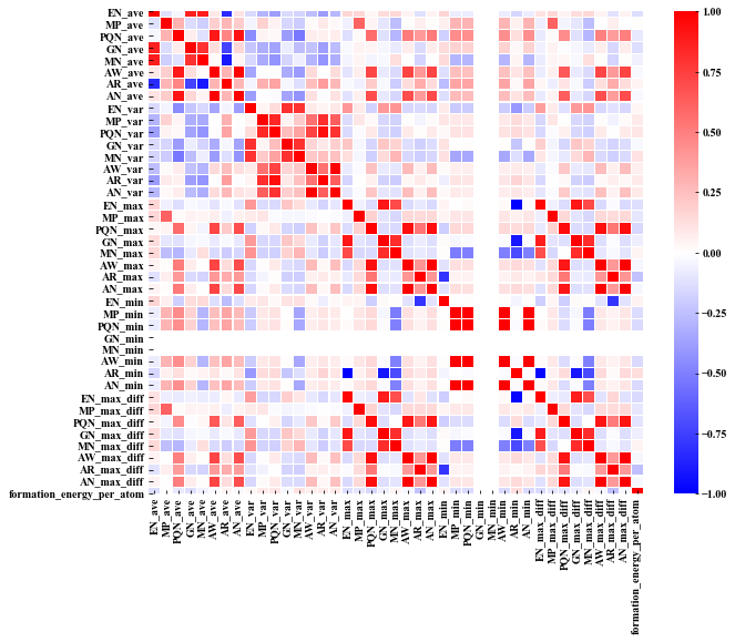
今回は、Li-O系の化合物についてのデータになっているため、GN_min(族番号の最小値)は、必ず１（Li）になり、また　MN_min(メンデレーエフ番号の最小値)も必ず１(Li)になるため、相関は0となっている（白色）。
また、記述子間で相関係数が高い（0.5以上）のものがいくつかあるため、多重共線性が発生してしまうと考えられる。

ちなみに、変数同士の相関係数だけを確認したい場合は、以下のようにcorr()を使用すると相関係数が取得できる。

df_corr = df.corr()
df_corr

まとめ

機械学習にかける前に、このような最低限のデータ分析を行うことが大切である。データ分析によって、新たな発見が、精度向上や知見を産むことが多々ある。また、異常値や物理的におかしい値などを発見することもできるため、それらを事前にすることも可能である。このようなテンプレートでも良いため、まずはデータ分析を行おう。